aamir.consulting math that moves the world in service of others

Piece 02

The Geometry
of Confidence

See which risks actually decide whether a project lands on time and on budget so you can act decisively ahead of time to mitigate them.

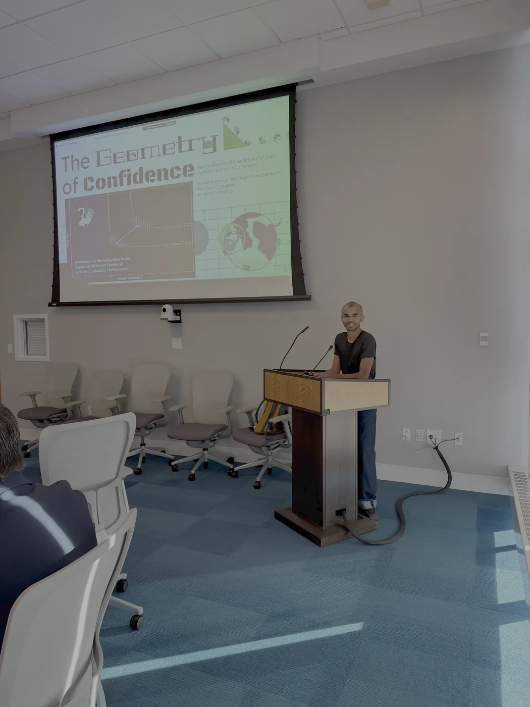
NASA Cost & Schedule Symposium · Glenn Research Center · LinkedIn Post

Frame · mirror · integrate · test

Aamir presenting The Geometry of Confidence at a podium, the title slide on the screen beside him — Presenting the method

Conference name tag reading NASA Cost and Schedule Symposium, Glenn Research Center, August 25 to 27 2026, Aamir Ahmad, aamir.consulting — Glenn Research Center · 25 to 27 Aug 2026

Aamir standing beside a full spacesuit on display at NASA Glenn Research Center — Good company

Problem

The Problem

Which risks will hurt the most, and by how much?

Teams and project managers need to know which risks in their project will matter most to cost and schedule, and they need to know it early enough to act decisively and mitigate them.

Response

The Response

A method that names the risks that matter, and a picture that shows why.

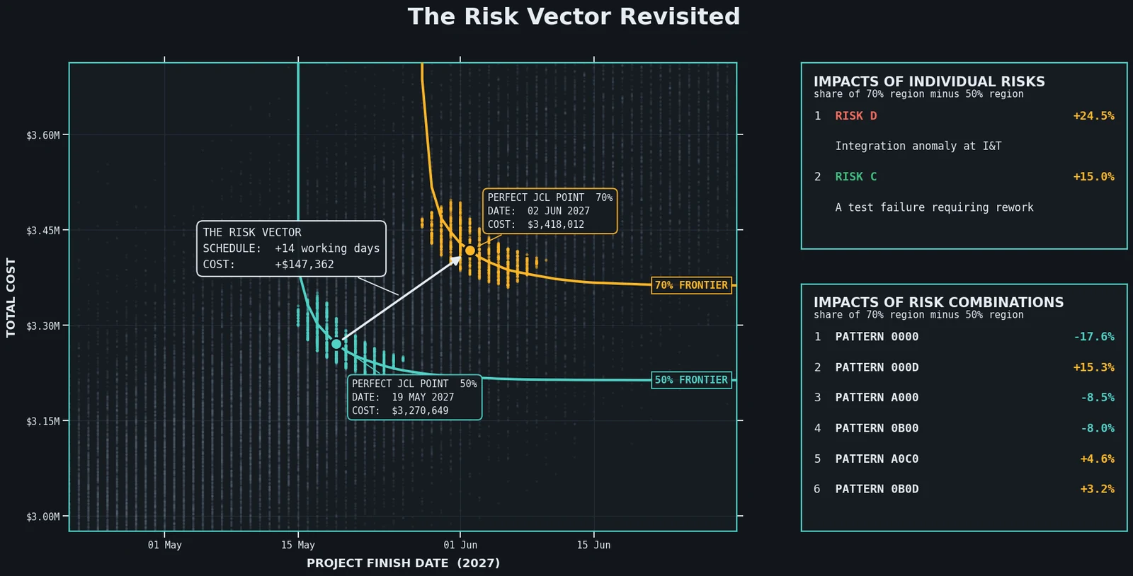
I built a method that points out the most consequential risks, and an intuitive graph that communicates both the consequences and the risks driving them.

The finished picture: the cost and schedule gap between two outcomes on the left, and the risks that account for it ranked on the right — Sneak peek The cost and schedule gap on the left; the risks that account for it, ranked, on the right. For the full method, read below.

Method

The Method

How it works, step by step.

The rest of this page builds the method step by step, on a worked example anyone can follow.

Framework: NASA Cost Estimating Handbook v4.0, with substitutions
Worked example: Archimedes' sun-laser: two subsystems, four risks, 140 simulated outcomes

The worked example is illustrative, not real programme data. The method came out of my work at NASA's Kennedy Space Center.

Premise

The question someone else asked first

Louis Fussell, 2024

At the 2024 NASA Cost and Schedule Symposium, Louis Fussell presented on the standardization of Joint Confidence Level (JCL) value selection. A JCL model describes the possible cost and schedule outcomes of a project through a Monte Carlo simulation built on initial schedule assumptions. Louis wanted to develop a confidence interval around the perfect JCL point. He wanted it for a good reason: to tie the JCL back to discussions about project risks.

That is the right instinct, and this work follows it. Where it ends up is somewhere other than a confidence interval, for reasons that take until the fourth section to become clear.

Part 1 · Baseline

Archimedes' sun-laser

two subsystems, four risks, one cost-loaded schedule

Archimedes is a mathematician in Syracuse, Sicily. Roman ships are headed to besiege the city, and he is going to build a sun-laser to defend it. The project has two subsystems: mirrors to focus the sun's rays, and a frame to move them.

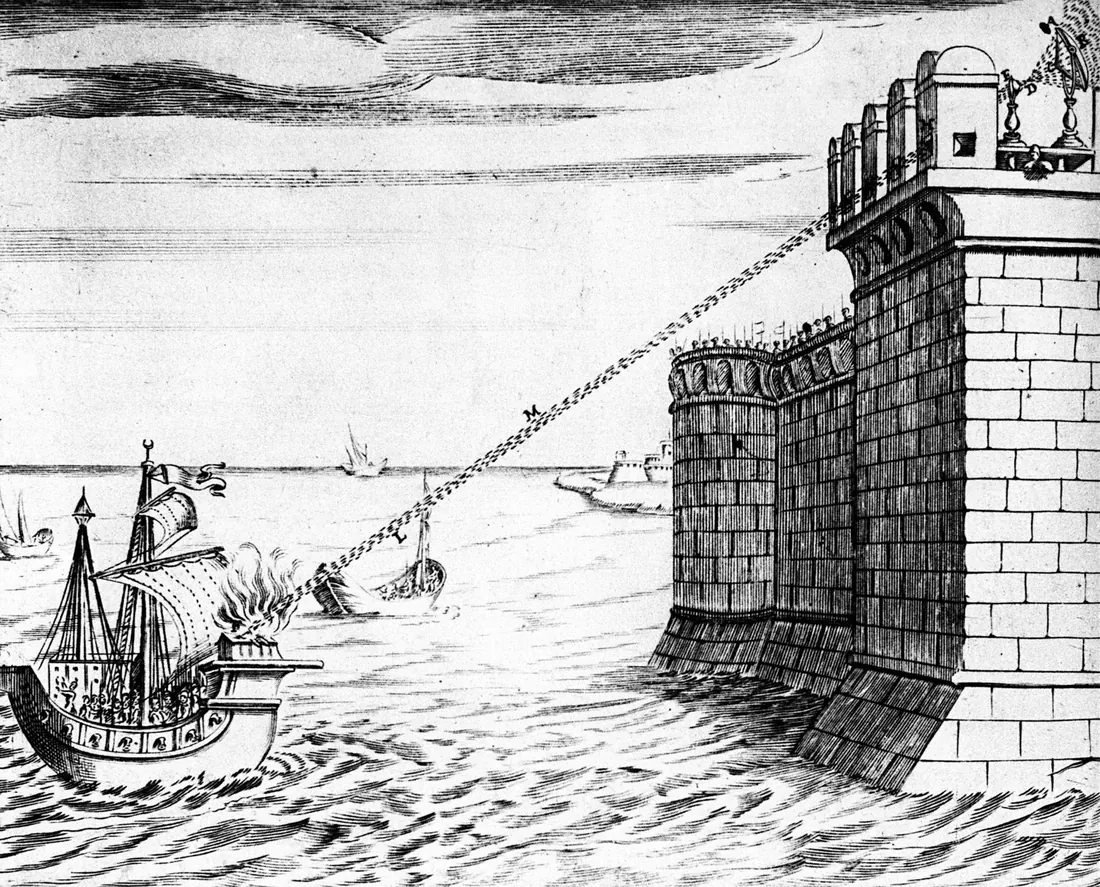
An old engraving of Archimedes' burning mirrors setting fire to Roman ships besieging Syracuse — Plate I The requirement. A toy project is the honest way to demonstrate a method: every number that follows can be checked against the schedule below, and nothing is hiding behind a real programme's complexity.

Design, build and test for each subsystem, then system integration and test. The schedule is loaded with costs, with three-point uncertainty on every task, and with four discrete risks. Two substitutions from the NASA Cost Estimating Handbook (CEH) baseline are worth naming: uncertainties are lognormal rather than triangular, and risks are modelled as schedule events carrying a probability below 1 rather than as cost reserves.

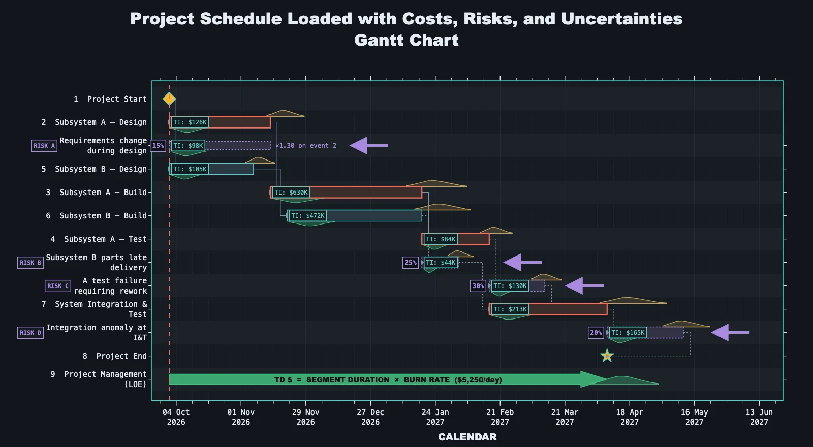
Gantt chart of the sun-laser project with task costs, lognormal uncertainty curves on each bar, and four risks annotated A through D — Fig 01 The cost-loaded schedule. Each bar carries its task cost and a lognormal duration distribution; project management runs as level of effort at $5,250/day, so schedule slip buys cost directly. The four risks sit in the rows marked A to D.

The four risks
Risk	Event	Probability	Cost impact
`A`	Requirements change during design	15%	$98K
`B`	Subsystem B parts late delivery	25%	$44K
`C`	A test failure requiring rework	30%	$130K
`D`	Integration anomaly at integration and test (I&T)	20%	$165K

Why the probabilities matter later Risk C is the likeliest at 30% and Risk D the second most expensive at $165K, but neither fact predicts which one separates confidence levels. That is the whole point of what follows: prior probability and cost impact are not the same as driving the difference between two outcomes a manager is actually choosing between.

Part 1 · Simulate

Run the Monte Carlo simulation

every iteration is one possible world

Each iteration samples a duration for every task, decides whether each risk fires, and resolves the schedule to a finish date and a total cost. Thousands of iterations make a cloud, and the cloud is the JCL.

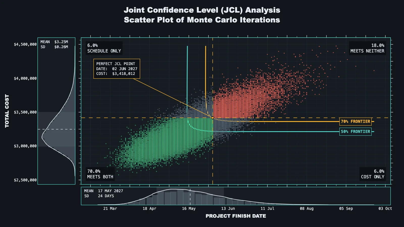
Scatter plot of Monte Carlo iterations in cost versus finish date, divided into four quadrants by the perfect JCL point, with marginal distributions on both axes — Fig 02 The perfect JCL point sits at 02 Jun 2027 and $3,418,012, and the quadrants around it are the answer a manager is handed: **70% meets both** cost and schedule, 6% schedule only, 6% cost only, 18% meets neither. The marginals show cost at $3.25M mean (SD $0.26M) and finish at 17 May 2027 (SD 24 days).

That single number, 70%, is where a conventional JCL analysis stops. It is also where the manager's real question starts: what would it take to be somewhere else on this cloud, and what is holding us here?

Part 1 · The Snag

Flexible thinking

the devil's in the details

Fussell's proposal was a confidence interval around the JCL point. Working through it, the idea runs into something that cannot be negotiated away.

Hmm…

Confidence intervals are statistical objects.

They describe uncertainty about a parameter estimated from a sample.

Wait!

JCL distributions are probabilistic constructs.

Confidence intervals have no meaning in this context.

The Monte Carlo cloud is not a sample drawn from a population; it is a simulated distribution generated from assumptions. There is no parameter out in the world that the cloud is estimating, so there is nothing for a confidence interval to be about. Adding more iterations does not narrow the interval. It just resolves the cloud.

So the honest answer to Louis's question is that the object he asked for cannot exist. The useful answer is to ask what he actually wanted it for: tying the JCL back to risk. That survives the objection intact.

Part 1 · The Table

A new data table

record which risks fired, iteration by iteration

The move is cheap and it happens while the simulation is already running. Alongside each iteration's cost and finish date, record the risks that fired in it: the individual risks (A, B, C, D) and the combination as a pattern (A0C0 means A and C fired, B and D did not).

Every point in the scatter plot now carries its own causal history. Which means that instead of asking for statistics about a parameter, we can report descriptive statistics for selected regions of the JCL, and read off the risk profiles that drive project performance to those cost and schedule levels.

Hmm…

Confidence intervals are statistical objects.

They describe uncertainty about a parameter.

Wait!

JCL distributions are probabilistic constructs.

Confidence intervals have no meaning in this context.

A-ha!

We can report the statistics of targeted regions.

We get the best of both worlds.

What changed Nothing about the simulation, and nothing about the JCL number. The only addition is bookkeeping, and it converts the scatter plot from a picture of outcomes into a queryable record of causes.

Part 2 · Regions

Choosing regions of the JCL to compare

two points, three candidate geometries, one that works

Start by choosing two points on the JCL scatter plot to compare, and build the regions around them. Here they are the perfect JCL points at the 70% and 50% confidence levels, the two options a manager is realistically weighing.

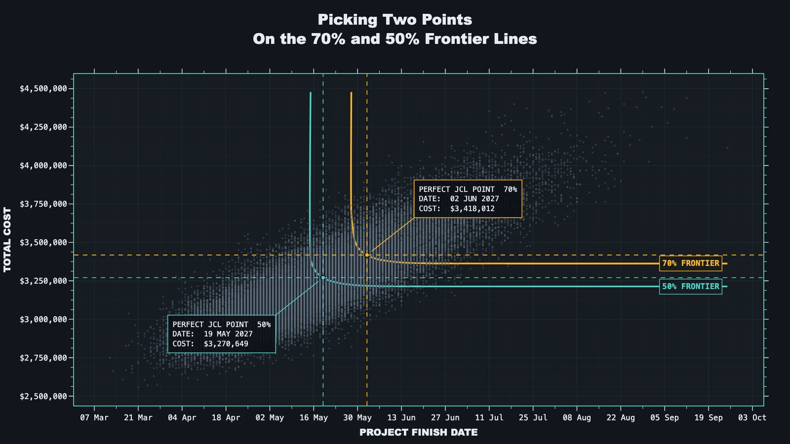
The scatter plot with the 70% and 50% frontier lines drawn and the perfect JCL point on each one labelled — Fig 03 The 70% point: 02 Jun 2027, $3,418,012. The 50% point: 19 May 2027, $3,270,649. Two weeks and about $147K apart. The question is what buys the difference.

A single point has no statistics; a region does. But a region has to be drawn, and how you draw it decides whether the comparison means anything. Three candidates, in the order they suggest themselves:

Confidence level bands

70%: 1,655 pts · 50%: 1,757 pts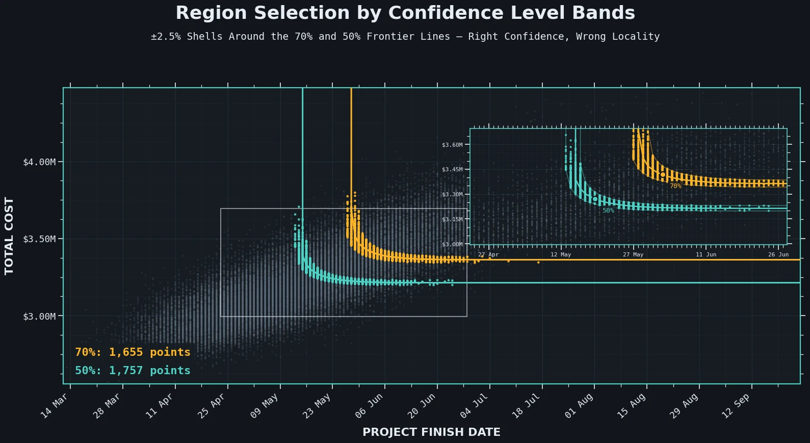

Thin shells drawn along the 70% and 50% frontier curves, sweeping the full width of the scatter plot — Fig 04±2.5% shells around each frontier line.

ProAll the points are at a similar confidence level.

ConDifferent parts of the band are not comparable to each other. A point at the far cheap-and-late end of the shell has nothing in common with one at the expensive-and-early end.

Elliptical neighbourhoods

70%: 6,403 pts · 50%: 9,130 pts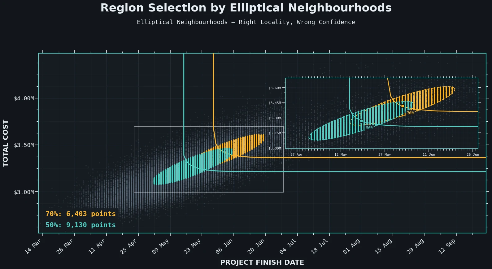

ProPoints within each region are statistically relevant to each other, because they are genuinely nearby outcomes.

ConThe points in the region are not all at a similar confidence level, so the comparison quietly mixes 70% outcomes with 60% and 80% ones.

The intersection: the best of both worlds

70%: 920 pts · 50%: 935 pts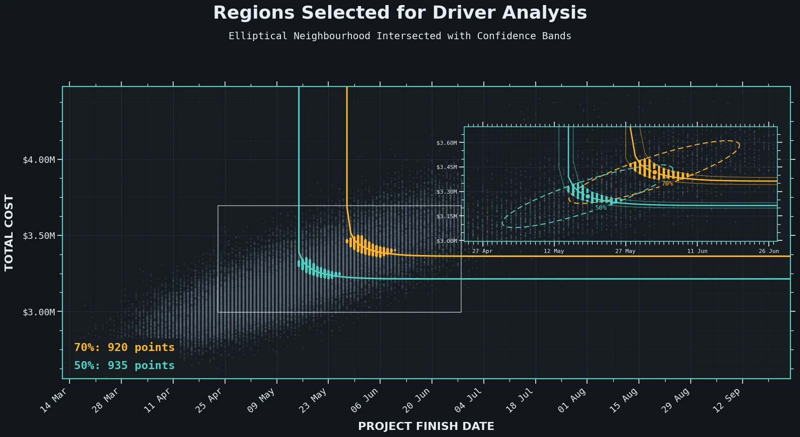

The elliptical neighbourhood intersected with the confidence band, leaving a small lens-shaped region around each point — Fig 06 Elliptical neighbourhood intersected with confidence band.

ProPoints in each region are statistically relevant to each other and at a similar confidence level. Both objections answered at once.

CautionThe intersection is small: 920 and 935 points here, down from thousands. Run enough Monte Carlo iterations to reach convergence, or the region will be describing noise.

Why this is the load-bearing decision Everything downstream is descriptive statistics on two sets of points. Choose the sets badly and the attribution is confidently wrong: right confidence and wrong locality, or right locality and wrong confidence. The intersection is the only one of the three that lets the two regions be compared on both terms.

Part 2 · Vector

The risk vector

we have the difference; we need to know what drives it

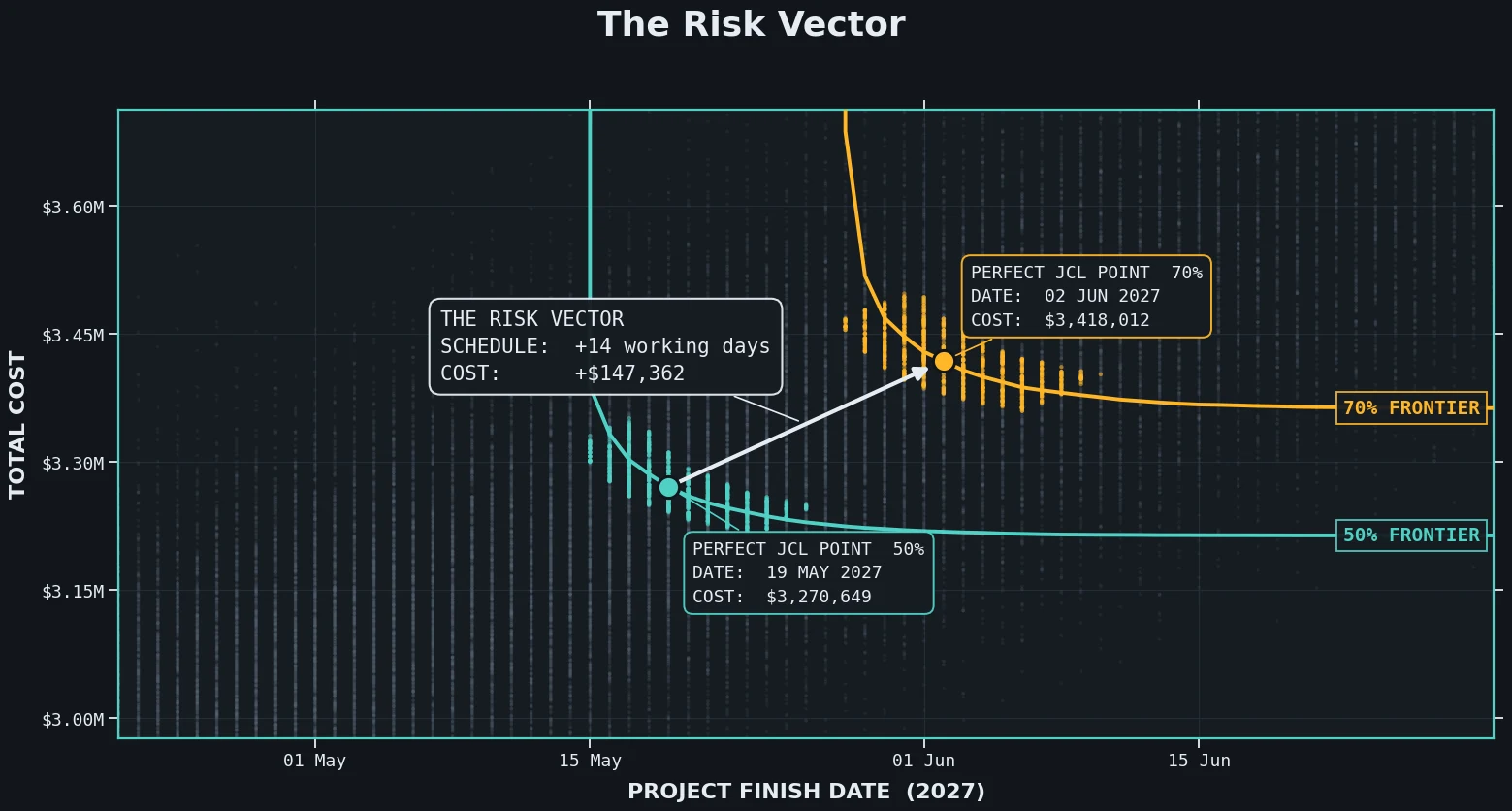
A white arrow drawn from the 50% point to the 70% point, annotated plus 14 working days and plus $147,362 — Fig 07 The arrow between the two points: **+14 working days and +$147,362**. That is the price of moving from 50% confidence to 70%.

The vector states the cost of the upgrade in the only units a manager cares about. What it does not say is what you are buying protection from. Since every point in both regions now carries the list of risks that fired in it, that question has an answer.

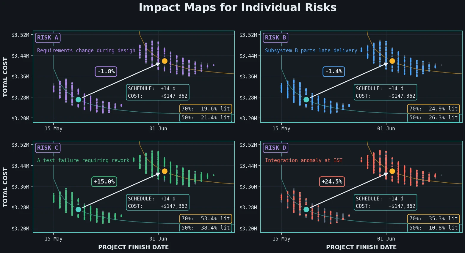
The measure is simple: for each risk, what share of the 70% region has it lit, and what share of the 50% region? The difference between those two shares is how much that risk separates the two confidence levels.

Part 3 · Drivers

Visualizing the impact of the risks

individually, then in chains

Individual risks

This is how the ranking at the top of the page is produced.

Four small panels, one per risk, each showing the two regions with the points where that risk fired highlighted, and the percentage-point difference between them — Fig 08 One panel per risk. The highlighted points are the iterations in which that risk fired; the figure in the box is the share of the 70% region minus the share of the 50% region.

Impacts of individual risks: share of 70% region minus 50% region
Rank	Risk	Event	70% lit	50% lit	Difference
1	`D`	Integration anomaly at I&T	35.3%	10.8%	+24.5%
2	`C`	A test failure requiring rework	53.4%	38.4%	+15.0%
3	`A`	Requirements change during design	19.6%	21.4%	−1.8%
4	`B`	Subsystem B parts late delivery	24.9%	26.3%	−1.4%

Amber: more common in the 70% region. Green: more common in the 50% region.

Read the bottom of the table too Risks A and B come out flat, slightly negative, which is noise around zero. They fire at much the same rate whether the project lands at 50% or 70%, so managing them does not move the project between those confidence levels. A JCL number alone cannot tell you that, and it is the kind of finding that changes where a manager spends attention.

Chains of risk

The same treatment applies to combinations. We can see how each risk combination contributes to changes in cost and schedule, and prioritize which chains of risk need managing.

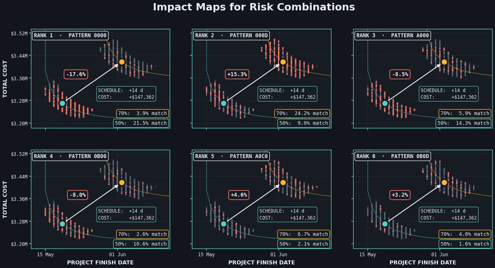
Six ranked panels, one per risk-firing pattern, each showing the match rate in the two regions and the difference — Fig 09 The six patterns that separate the regions most, ranked by the size of the difference. `0000` is the pattern where no risk fires at all; `000D` is D alone; `A0C0` is A and C together.

Impacts of risk combinations: share of 70% region minus 50% region
Rank	Pattern	Meaning	70% match	50% match	Difference
1	`0000`	No risk fires	3.9%	21.5%	−17.6%
2	`000D`	D alone	24.2%	9.0%	+15.3%
3	`A000`	A alone	5.9%	14.3%	−8.5%
4	`0B00`	B alone	2.6%	10.6%	−8.0%
5	`A0C0`	A and C together	6.7%	2.1%	+4.6%
6	`0B0D`	B and D together	4.8%	1.6%	+3.2%

Amber: more common in the 70% region. Green: more common in the 50% region.

The top of this list is the clean-run pattern, and it points the other way: a project that lands at 50% confidence is more than five times as likely to have had nothing go wrong as one that lands at 70%. Read together with rank 2, the story is a single sentence: the 70% region is where the integration anomaly fires and the project absorbs it, and the 50% region is where the project needed a clean run to get there.

The risk vector revisited

A simple way to summarize which risks drove the difference between the two regions.

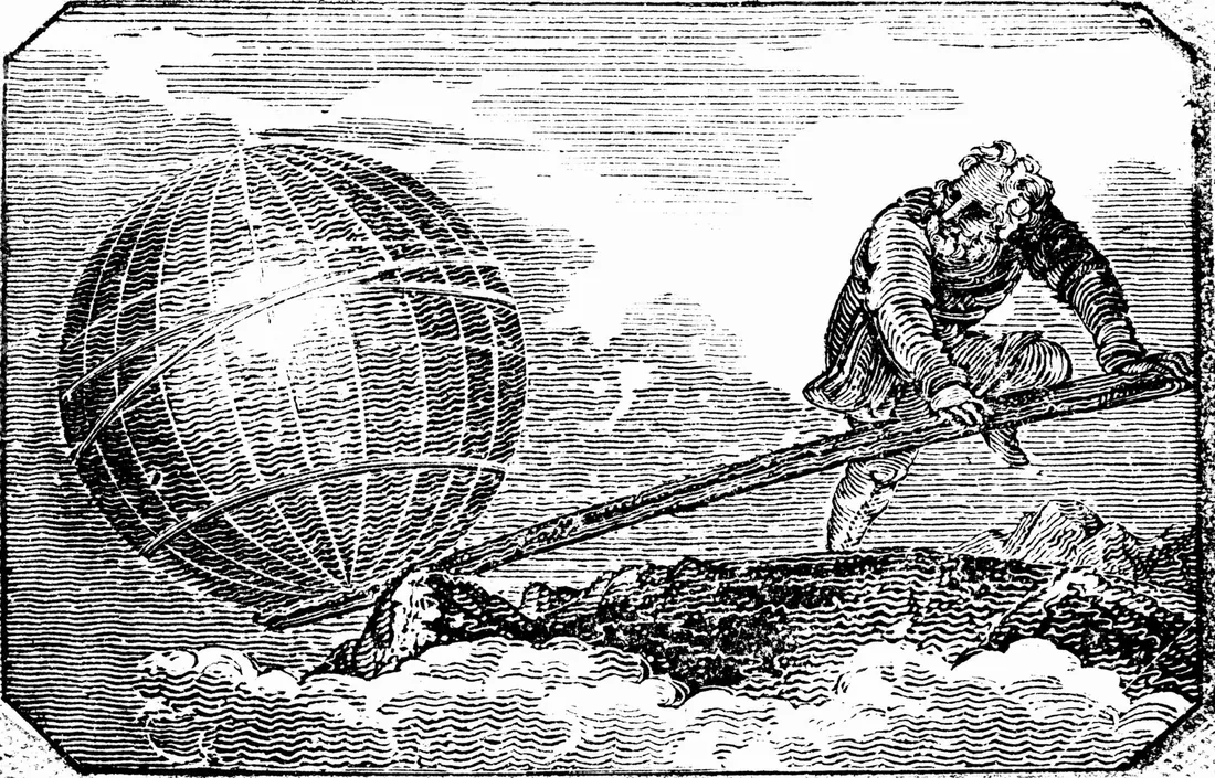
The risk vector plot with two summary panels beside it ranking the individual risks and the risk combinations by their impact — Fig 10 The whole argument on one slide: the price of the upgrade, and the register of what it buys, ranked.

Archimedes finished his sun-laser ahead of schedule and under budget, and turned his attention to moving the Earth with a lever and a fulcrum.

An old engraving of Archimedes levering the Earth with a long pole — Plate IIGive me a place to stand.

Sources

References

the framework, and the question that started it

Framework National Aeronautics and Space Administration. (2015). NASA Cost Estimating Handbook (Version 4.0). NASA Headquarters.
Premise Fussell, Louis (2024, April 23). Standardization of JCL value selection [Conference presentation]. 2024 NASA Cost and Schedule Symposium, Hampton, VA, United States.

Need to know which risks to act on before they cost you?

Bring me the decision in front of you. I will show you which risks decide the outcome, and where your budget and schedule buy the most protection.

Start a conversation

The Geometryof Confidence